The list that every artist dreams to make – Billboard Hot 100 has seen all of the greatest artists of our time top its charts: The Beatles, Stevie Wonder, Whitney Houston, Queen, ABBA, Michael Jackson just to name a few. To join this star-filled elite is no small feat as it requires a single to be the number one hit for a week.
It may come as no surprise that there are a few dominant genres that top the charts constantly, after all this is the Hot 100 chart and mainstream genres are well… mainstream. Check out the following analysis of the Billboard Year-End Hot 100 charts from 2006 to 2019 and how our music taste has evolved.
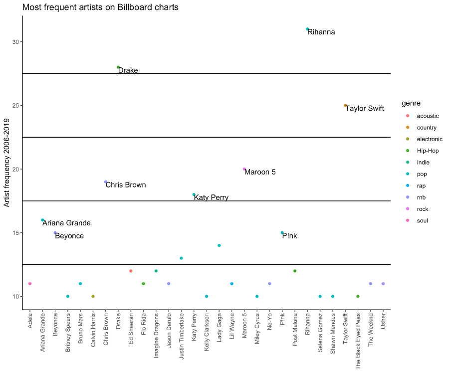
Plot 1. All the artists with 10 or more songs on the Billboard charts throughout 2006 – 2019.
Recently the genres have become more difficult to distinct and label, with the likes of Lil Nas X and Post Malone releasing songs within variety of genres.
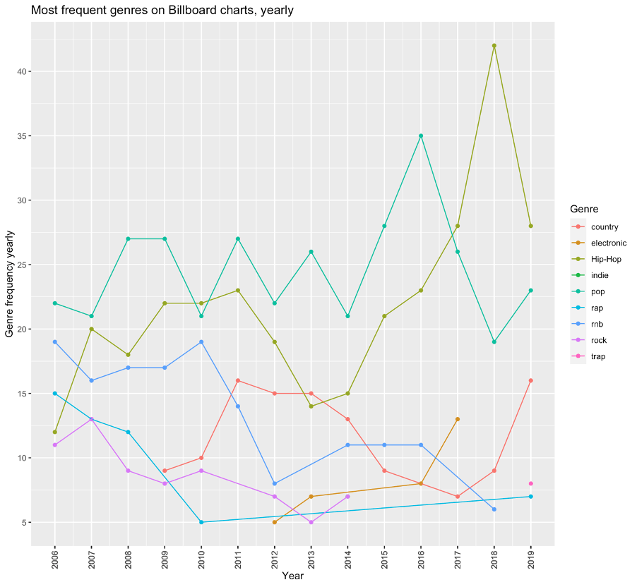
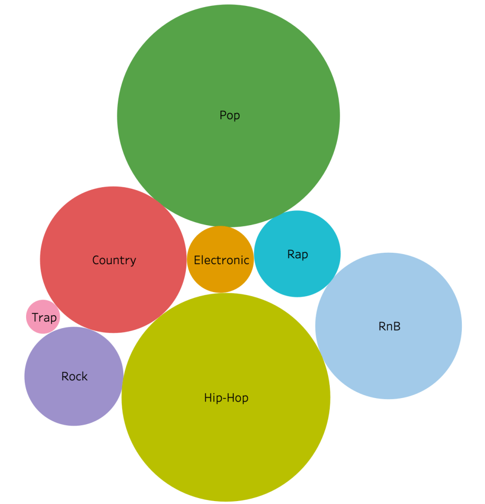
Plot 2. Genre frequency on the charts, yearly.Plot 3. Genre frequency on the charts, in total.
This is my empirical bachelor’s thesis in developmental economics. For better reading, references and appendix please view the pdf file below.
1. Introduction
Corruption is a phenomenon that many would argue has bad connotations. There seems to be a consensus that corruption is unwanted and something that should not exist. Among researchers and economists, there is ambivalence about the real effects of corruption. The issue of corruption has divided many researchers into two groups: those who think that corruption “greases the wheels” and those who think that corruption “sands the wheels” of economic growth. In the ongoing discussion, the former group believe that some corruption can lead to improved efficiency whereas the latter reject that claim altogether (see Bardhan (1997) for a great summary).
Most of the research in the field focuses on how corruption affects growth directly and through channels such as investment. This research looks at different qualities that countries possess that might explain what contributes to corruption; such as wealth measured as GDP, education levels, bureaucratic efficiency, judiciary efficiency, openness to trade, political stability, cultural differences, and others. Most research done on Foreign Direct Investment (FDI) examines how much corruption, among other variables, affect it. In contrast, research on foreign aid looks at how foreign aid influences corruption. However, there is little research on how FDI impacts corruption, especially FDI and foreign aid simultaneously. There seems to be a consensus that poorly developed countries are among the most corrupt as well as among those who receive most foreign aid. Due to a lack of data on these countries, not much research has been done. This sparked a natural interest and is the motivation behind this paper. The United Nations (UN) list of least developed countries is used to pick out the countries observed and are defined as: “LDCs are low-income countries suffering from the most severe structural impediments to sustainable development”. The research question of interest is as follows: “How do foreign funds impact corruption in the least developed countries?”
The current study draws on empirical evidence and insights of theories proposed in the literature to create an empirical model. This paper contributes to the literature by examining the simultaneous effects of FDI and foreign aid on corruption by using a panel and cross- country data on two models: fixed-effects regression and OLS regression. Contrary to previous research insufficient evidence is found on the negative relationship between corruption and investment, and corruption and foreign aid. However, a strong judiciary efficiency effect on corruption is found.
The paper is structured as follows. Section 2 looks at the various theories and evidence presented behind corruption. Section 3 presents the main data and lays out the empirical model. Section 4 describes the cross-section and panel data regression results and discusses. Section 5 concludes.
2. Theoretical background
In the literature, many determinants of corruption have been suggested; they can be categorized into three branches. The first branch takes an economic approach explaining corruption with various measures of growth, trade, resources, expenditure, etc. The second branch takes a political approach and looks at judiciary efficiency, bureaucracy, rights, freedom, and so on. The final branch is cultural, and encompasses cultural dimensions, ethnicities, language, schooling, colonial history, etc. One determinant that comes up repeatedly and is common in all branches is wealth measured as GDP. Many of the studies look at some combination of those branches. In this paper, the focus is on the economic approach in combination with the political approach.
The United States was the first country to outlaw foreign bribery in 1977 and remained the only one until 1998, when it was brought up globally at the OECD Anti-Bribery Convention. Hines (1995) studied the effects of the American bribery ban and found that US investors, relative to others, invested less in more corrupt countries. However, the conclusion was that the overall corruption likely remained unchanged simply because other foreign investors took their place. For a long time, there was little doubt and evidence that a corrupt country could have a fairly stable long-term growth. Countries such as China, Thailand and Indonesia have put that to the test as they have continued to enjoy solid levels of growth despite relatively high corruption rates. A possible explanation for this is the nature and predictability of corruption (Campos et al., 1999; Sheifler & Vishny, 1993; Wei, 2000). If there is a centralized bribe system that can efficiently maximize aggregate bribes, enforce action, and penalize officials who deviate from the agreed bribe level, corruption can be efficient in the second- best world (Sheifler & Vishny, 1993). Nonetheless, Campos et al. (1999) finds clear evidence that, independent of the degree of predictability, more corruption equals less investment.
Due to a lack of consistent and reliable data, corruption had been largely theoretical and explained mostly through principle-agent theory up until the mid-1990s. Leff (1964) was among the first to study corruption and is considered to be one of the most influential advocates of the view that corruption can be efficiency-enhancing. He argues that in a state with an inefficient government that imposes rigidities, “speed money” or “grease money” can be used to remove or lessen those obstacles and promote investment. Along similar lines, Bayley (1966) argues that individuals who oppose government policies may make it work for themselves through corrupt behavior. He touches on the cultural differences regarding the definition of corruption and argues that what is considered corrupt behavior in the Western world is considered moral and expected transaction in other places. Both Leff (1964) and Bayley (1966) provide very little evidence, if any, and mainly anecdotal. Tanzi (1998) argues against their sentiment, showing that government stringencies are not exogenous and can be changed. He suggests that rigidities might be constructed to extract bribes and could lead to a cycle of more rules and more corruption.
Among the more recent advocates of grease hypothesis, Meon & Weill (2010) show that corruption has a negative but insignificant effect on developed countries with efficient institutions but show that it has positive effects on countries with an inefficient government. They suggest that letting corruption grow in such countries might increase growth, however, they caution that such a strategy is risky and in the long run, will most likely lead to more inefficient governance. Aidt (2009) opposes that finding by arguing that corruption has less effect on growth in poorly governed countries merely because it cannot get much worse.
Among those who support the “sands the wheels” hypothesis, the seminal work of Mauro (1995) stands out the most. He pioneered the empirical cross-section data research on corruption and found significant evidence that corruption causes investment rates to fall and, in turn, slow down economic growth. Not only corruption level but the predictability of corruption is negatively correlated with investment (Campos et al., 1999; Wei, 2000). High GDP per capita reflects high consumption potential and is attractive to foreign investments, therefore some correlation can be expected between the two variables. The significant negative correlation that GDP per capita has with corruption is very evident in the literature (Ades & Di Tella, 1999; Robertson & Watson, 2004).
A country open to trade is more likely to receive more investments and face more competition. This competitive pressure can drive out monopolistic rents and, with that, corruption (Ades & Di Tella, 1999; Leite & Weidmann, 1999). They argue that restrictions on foreign trade can create increased rents and rent-seeking behavior. Similarly, Sheifler & Vishny (1993) argue for competition as a way to drive out rents in a bureaucracy within the confines of a country. Trade openness can therefore be seen to fit similarly with FDI for better estimation of corruption.
Foreign aid research on corruption shows mixed results. Alesina & Weder (2002) examined if less corrupt countries receive more bilateral aid- the results turned out inconclusive. They find an insignificant positive correlation that corrupt countries receive more aid. This interesting finding could be explained with some political, historical, and cultural agendas of the home countries. On the contrary, Tavares (2003) finds significant evidence of the opposite to be true. He suggests that aid is usually given if the rules are followed and conditions met, and that aid alleviates budget shortages which can increase salaries for public servants.
Judiciary efficiency and rule of law is a good checks-and-balances system in a country to keep corruption down. An efficient system should be able to account for foreign aid and penalize the misuse of funds. The effect of both could have a stronger impact on corruption. A strong rule of law and judiciary system is found to be correlated negatively with corruption and dampen it (Brunetti & Weder, 2003; Leite & Weidmann, 1999).
3. Data and empirical strategy
From the literature and theory review above, five determinants are chosen. The lion’s share of the data listed below is downloaded from The World Bank for years 2007 to 2017 (unless specified otherwise). First and foremost, the list of countries chosen for this study are the least developed in the world according to the United Nations. For countries to make the list they must meet or be below certain criteria of human and economic development. Being on the list grants those countries exclusive access to international support measures (UN, 2020). The list is revised every three years and new countries can be included in the list or graduate from it. During the 11 years from 2007 to 2017, 46 countries remained on the list. Although, thirteen of them had to be dropped due to missing data, resulting in 33 countries. The full list of countries included in this study is shown in Appendix A.
3.1.Measures of corruption
Measuring corruption is a tricky task. It is extremely difficult and costly to obtain data on actual corruption namely because it is not publicly available; people hide corrupt practices because they are not considered ethical. This is the reason why nearly all research done on corruption uses corruption perception indexes. Those indexes do not measure corruption per se, but the perceptions of businesspeople and country experts. Aidt (2009) exercises the thought that those perceptions can be problematic because they may be biased by observed economic performance and therefore be negatively correlated with economic growth, making the validity of previous findings somewhat questionable. Olken (2009) conducted extensive research on actual versus perceived corruption in Indonesian villages. In his research of over 400 road projects and villages, he finds that locals are good at observing inflated prices in these projects but fail to do so when quantities are artificially increased. What’s interesting is that he observed several individual biases such as education level and ethnography. He finds little positive correlation between actual corruption and perceived corruption and suggests using corruption perception data with caution.
Various indexes of perceived corruption are used in research such as The International Country Risk Guide (ICRG), Business International (BI), World Competitiveness Report (WCR), World Bank (WB) and Transparency International (TI). The last two are among the most widely used in recent research. To make this analysis more robust, I have decided to go along with the two as they share a similar definition and therefore make for a good between comparison. In short, they are both defined as “use of public power for private gain”.
The first index is the most well known and most widely used, it has been released annually by Transparency International and measures public sector corruption perceptions (CPI). It encompasses up to thirteen surveys conducted by twelve credible institutions that survey a substantial amount of countries at least once every other year. To be included in the ranking the country has to be covered by at least three surveys. The index is scaled from 0 to 100 and ranges from highly corrupt to very clean. To make it more intuitive this data is inversed that, in this paper, a higher score means higher corruption and vice versa.
The second index, Control of Corruption (CC), is constructed by The World Bank as a part of their Worldwide Governance Indicators. It summarizes information from over thirty data sources and combines the views of enterprises, citizens, and experts in the public sector. It measures the perceived extent to which public power is used for private gain annually. Originally, it is scaled from -2.5 being most corrupt to 2.5 being least corrupt. Again, for intuition and easier comparison reasons, the data is rescaled and inversed. Therefore, in this paper, it subsequently ranges from 0 (least corrupt) to 100 (most corrupt).
3.2.Measures of FDI and foreign aid
Data for both Foreign Direct Investment and foreign aid are gathered from The World Bank for the period 2007 to 2017. FDI, as discussed above, has been extensively researched in the context of corruption. The World Bank (2020) defines FDI as: “net inflows of investment to acquire a lasting management interest in an enterprise operating in an economy other than that of the investor.” The measure of net FDI inflows as a percentage of GDP is used in this study. This data is limited in that it does not include capital raised locally which, according to WB, is an important source of investment financing in some developing countries. Therefore, it does not give a complete picture of international investment in an economy.
The measure used for foreign aid is the net Official Development Assistance (ODA) as a percentage of Gross National Income (GNI). This ratio is a good measure of how dependent countries are from aid. According to WB (2020), ODA consists of disbursements of loans made on concessional terms and grants to promote economic development and welfare. It includes loans with at least 1⁄4 of grant element. The data can be somewhat misleading as it does not take into account aid given by countries, so some countries who give more than they receive still show up as net aid receivers. However, for our analysis, it is not a likely problem as the sample consists of least developed countries. Another problem that may arise is that some countries traditionally receive large amounts of aid which reveals both interests of the donor and the needs of the recipient, therefore WB cautions when drawing policy conclusions.
3.3.Other variables
Various forms of wealth measurement are used in corruption research, most often it is GDP. In this paper, GDP per capita is based on purchasing power parity is used for better comparison between countries as the dollar value has the same power in each country. GDP is the sum of total value added and product taxes less subsidies in an economy for a certain time-period, usually a year. The natural logarithm is taken to reduce any possibility for positive skewness, and it is a better proxy for growth comparison.
Trade openness is a variable that measures the sum of exports and imports as a percentage of GDP. It shows the exposure a country is facing in international trade.
Rule of law is another perception-based measure which means it is likely to be influenced by individual biases. The World Bank (2020) defines it as: “perceptions of the extent to which agents have confidence in and abide by the rules of society, and in particular the quality of contract enforcement, property rights, the police, and the courts…”. It ranges from approximately -2.5 (low confidence) to 2.5 (high confidence).
3.4.Specification
The main model in this paper is presented in Equation (1) and is a fixed-effects model:
where a is the fixed effect intercept unique to a country, beta are the common slope coefficients, i and t represent a country and a year respectively, and μ is the error term. CORR is either of the corruption perception indexes, FDIpct is FDI as a percentage of GDP, FAIDpct is the percentage of foreign aid as a percentage of GDP, LogGDPpc is the natural logarithm of GDP (PPP) per capita, TRADE is trade openness and RULE is rule of law.
The main focus is on the significance and sign of beta1 and beta2 and is expected to be negatively correlated to the dependent variable. The minus sign on the variables should tell us that an increase in Foreign Direct Investment and foreign aid should equal decreased corruption. Log of GDP per capita is expected to be significantly negative, implying that an increase in GDP would mean a reduction in corruption. Trade openness is expected to have a negative sign, as increased competition should lower corruption. Rule of law is expected to be negative as stronger judiciary system is expected to deal with corrupt behavior. However, causality will not be assessed and the question of what influences what remains open.
Moreover, for robustness, a second model is estimated using the Ordinary Least Squares (OLS) method where time-series are dropped and instead, the 5-year average of data is used. The determinants are the same as for Equation (1) except two additional variables are added, which were assumed to be constant over short periods and therefore could not be used in the fixed-effects model. The first variable is natural resources because resource richness in poorly developed countries is known to positively correlate with corruption (Lambsdorff, 1999; Tanzi, 1998). The second variable is ethnic fractionalization and measures ethnic diversity within a country (Mauro, 1995). It is expected to be positively correlated.
3.5.Econometric methodology
The dataset for this analysis is strongly balanced. Several tests for heteroskedasticity and autocorrelation show the presence of both. The most appropriate model for this panel data is the fixed-effects model, as it omits country-specific factors that are time-invariant (country fixed effects) such as culture to avoid omitted variable bias (Stock & Watson, 2005). The model is adjusted by clustering standard errors, so the estimations are more precise and robust in the presence of autocorrelation and heteroskedasticity over time within a country (Stock & Watson, 2005). The problem with this model is that any time-invariant variables, such as ethnic fractionalization index that remains constant, cannot be taken as an explanatory variable- therefore some possible information is lost.
Stock & Watson (2005) name the following four assumptions for this model (pp. 411-412). First, the error term has conditional mean zero for a country in the sample for all determinants over all periods, meaning that it does not depend on any values of determinants of a country in the sample, hence no omitted variable bias. Second, the distribution of variables for one country are identical to, but independent of, the variables for another country (e.g. simple random sampling). Sample in this paper although taken from a list is randomly selected. The third assumption states that large outliers are unlikely as the estimator can be sensitive to it. Lastly, no perfect multicollinearity is assumed, meaning that regressors should not be perfectly linear with each other.
The main model in Equation (1) is estimated using the fixed-effects model with clustered standard errors with both Transparency International and World Bank corruption indexes. Thereafter a regular OLS model with 5-year averages of the data for the period 2013 to 2017 is estimated for robustness and result comparison.
4. Estimation results and discussion
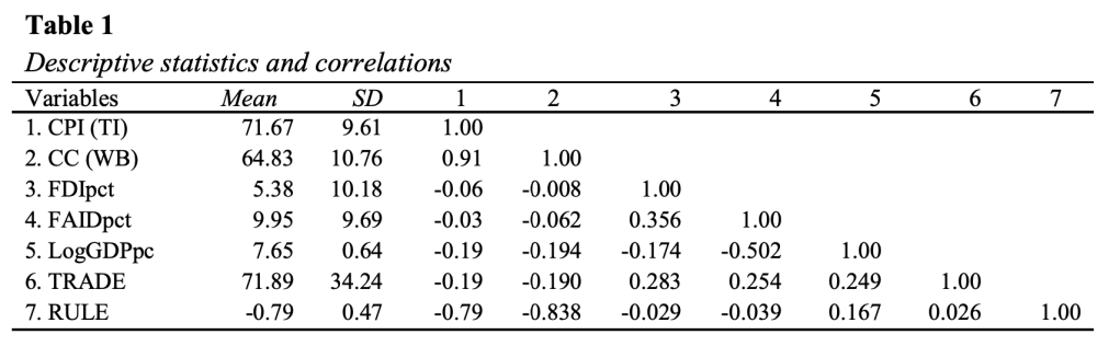
The mean, standard deviation, and correlations between variables are provided in Table 1. The high positive correlation between the two corruption perception indexes suggests that perceptions are somewhat similar and might be in the ballpark of actual corruption. Rule of law seems to have high explanatory power as it highly correlates with dependent variables. LogGDPpc is somewhat correlated with FDI and foreign aid which was expected.
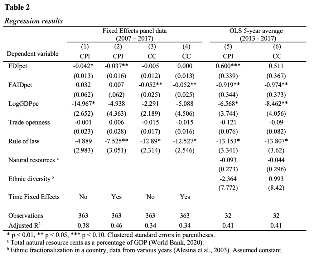
Table 2 presents panel data and cross-section regression results. The first four columns estimate data over the 11-year span for 33 countries. The last two columns take a 5-year average of data for years 2013-2017 and include 32 countries.
Regressions (1) and (2) use the Transparency International corruption index and show support that foreign investment is negatively correlated with corruption as anticipated. The coefficients are highly significant but rather small, meaning a one percent FDI increase is associated with a tiny decrease in corruption perception. On the other hand, foreign aid has an unexpected positive sign, though the coefficient is not significant. This can potentially be explained by the fact that a lot of foreign aid is given regardless of corruption levels, whereas for investors a corrupt government can lead to investments being placed in a different country. Interestingly, the coefficient on GDP drops three times and loses significance between the two regressions when we control for time fixed effects. This seems to indicate that over time GDP and corruption trend differently in our sample, meaning that as corruption decreases, GDP rises. The coefficient on trade openness is tiny, possibly due to FDI and GDP accounting for much of the information. Rule of law is negatively correlated as expected and significant at the 5% level when controlled for time effects, and close to significant at 10% when not.
The picture is somewhat different for the two variables of interest in regressions (3) and (4), which use The World Bank corruption perception index. FDI is still negatively associated although it has become even tinier and lost significance. The signs are, however, in line with previous research. In turn, foreign aid has become negative and significant at 5% levels. This seems to echo Tavares (2003), who found that foreign aid is associated with decreased corruption. The coefficients are rather small and do not suggest any real decrease in corruption. More interestingly, GDP is insignificant which is in stark contrast to most previous research. The signs, however, are appropriate and as expected, which suggest some validity. Rule of law has increased quite a lot and is now highly significant at one percent levels. It should be noted that there might be some bias involved as CC and rule of law indexes are constructed from many of the same sets of surveys. However, it suggests that a one-point increase in the rule of law index (measured -2.5 to 2.5) is associated with around a 12.5-point decrease in corruption perceptions. To illustrate, if the Central African Republic, who score the lowest on rule of law of all countries in this study, increased its judiciary efficiency to the level of Norway (second most efficient), it would experience a decrease in corruption to the level of France.
Regressions (5) and (6) use Transparency International and The World Bank indexes respectively and show more or less similar results. Very surprisingly, they show a positive correlation between FDI and corruption. What’s even more surprising is that in regression (5) this association is significant at 10% levels. Perhaps some strong swings in FDI percentage, due to different economic events, impact this result. Some backing for the negative correlation of foreign aid is found and is significant at 5% levels. Further on GDP has gained significance at one and five percent levels confirming findings in the literature. Rule of law continues to be highly significant suggesting even higher changes of corruption with an increase of judiciary efficiency. Out of the additional two variables, the sign on natural resources is surprising and suggests, in contradiction to previous findings, that more natural resources are associated with less corruption. A possible explanation might be that more rents from natural resources could increase wages in the public sector and decrease low-level corruption (Sheifler & Vishny, 1993).
5. Conclusion
This paper has studied different predictors of public sector corruption in the least developed countries in the world with a special interest in FDI and foreign aid. Two constraints on the study stand out. First, the lack of data on many of the LDCs has limited the size of this research. Second, this study is based on perception indexes which are likely not precise in showing actual corruption. I do not find sufficient evidence to claim that FDI decreases or increases corruption. Similarly, although more consistent than FDI, no conclusive results were found that foreign aid decreases corruption. This study does, however, find quite strong evidence on the negative correlation between corruption and judiciary efficiency. For example, if the Central African Republic were to improve their rule of law to the level of Norway, their corruption perception level would improve to that of France. The problem that arises here is that the rule of law is another perception-based measure that is likely biased, therefore it should be interpreted as such. That being said, this paper does not try to assess or suggest any type of causality, leaving that question open.
Future research should look at inter-country flows to determine more precise relationships and rule out any cultural and historical host-to-home country biases that could influence the data. Better understanding those biases and eliminating them should provide more information of the causal relationships. The biggest anchor in corruption research so far has been the measurement of corruption itself. While corruption perception indexes are the best measure we have, a full and clear picture cannot be drawn without actual data, in turn any policy suggestions can be misleading. The process of gathering actual data may be expensive due to the secret nature of corruption, but until objective data is available one should be cautious when interpreting these results.